Introduction

Digital Image Processing is a popular subject to study, it is taught in many universities for Computer Science Degrees and others have it as an elective. Here, we will understand how images are represented on the computer and modified to get the desired results using various techniques. We will mostly understand the gray-level images (informally called Black and White images). If you want to study this subject, I would recommend reading: "Digital Image Processing" by Rafael C. Gonzalez. It's a beginner-friendly book. I will also show some code in this blog. Let's jump into it!

Different ways to Import images in Python

We save images in JPG/JPEG, PNG, GIFs (a sequence of images), and HEIC which have their own benefits depending upon your requirements. But when we do processing on images we represent images using a matrix, if we have a colour image there will be 3 matrices depending upon representation, but when we import an image in Python using OpenCV we read it as BGR (Blue, Green, Red) (or RGB format).

Your system should have OpenCV installed using pip command

Write this command on your terminal (assuming you already have pip installed)

> pip install opencv-python

import cv2 as cv

# Reading Image using cv.imread()
img = cv.imread("OpenCV Python\img.jpg")        # Relative Path
# We can also give absolute path

We can also read images in Gray-Level Images (informally called Black and White images), Gray-Level images only have one matrix.

im_gray = cv2.imread('gray_image.png', cv2.IMREAD_GRAYSCALE)

We can convert BGR/RGB images to Gyar-Level using the simple formula :

Gray = (0.299 * Red) + (0.587 * Green) + (0.114 * Blue)

Code :

# Reading Image using cv.imread()
img = cv.imread("OpenCV Python\img.jpg")

# Python have BGR Format (not RGB)
# Seperating the matrices
B = img[:,:,0]
G = img[:,:,1]
R = img[:,:,2]

# converting to gray level image
gray = 0.299*R + 0.587*G + 0.114*B
gray = gray.astype(np.uint8)

or, we can simply use the inbuilt function in OpenCV :

# Using Built-in Function
gray = cv.cvtColor(img,cv.COLOR_BGR2GRAY)

To display images in Python using OpenCV, we use the cv.imshow() function. This function displays the image in a new window.

We also have to use cv.waitKey(0), which means do not close the window until any key is not pressed (KeyboardInterrupt). If we do not use this, then after the code is finished, the window closes automatically.

Code :

cv.imshow("Gray",gray)
cv.waitKey(0)

Demo :

Without cv.waitKey(0)

With cv.waitKey(0)

Now, let's understand what these image matrics are and how can we manipulate them.

Representation of Images in Matrix Format

Now, that we have imported images in our code, let's see how these images are represented. As we discussed BGR/RGB has 3 matrices (1 matrix for each colour) and if we have a gray-level image we have only 1 matrix.

Now, let's talk about what is stored in these matrices. Values can be understood as a pixels in the image. The value is a positive integer which represents a colour, every value represents a different color.

So the range of these integer values depends on the size of each pixel. Like most of the gray-level images each pixel size is 8-bits (8-bit unsigned integer) means values can range from 0 to 255 (binary : 0 -> 00000000, 255 -> 11111111), and 0 represents the pure black colour (no light) and 255 represents pure white (full light). We can infer these values as the intensity of light coming out from that pixel. So, 0 means no light, and 255 means full light.

See the image below as an example of the above topic,

Similarly, RGB images with a tuple of 3 values of 8-bit (each pixel takes 24 bits), eg, (200,34,34) looks red.

Also, we can make 8-bit to 5-bit if we want to reduce the size of the image but this may lead to loss in image quality. Also, we can make images of large size as 32-bit pixel size or more depending upon our requirements but the standard is to keep it 8-bit.

You can also print these image matrices on the terminal and understand them better.

Histogram

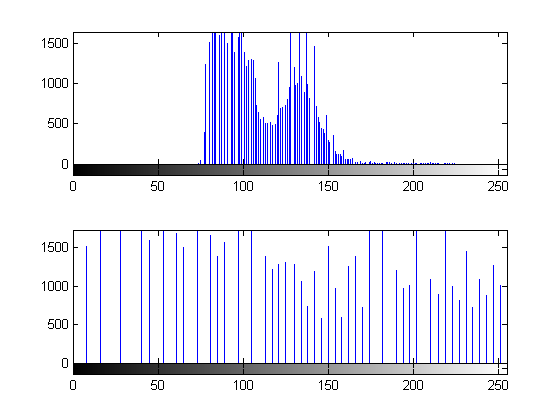
In simple terms, a histogram is a graph that shows the frequency of every gray-level value (count of no. of pixels with a particular gray-level value in the image matrix).

It's a very important topic in image processing. It has various applications like adjusting brightness, histogram equalization, etc.

Let's see the code for getting a histogram of the image matrix,

# Gives numpy array of histogram of 8-bit gray level image
def get_hist(gray):

    (rows,cols) = gray.shape

    # Calculating histogram of the given gray level image
    hist = np.zeros(256,dtype=np.uint32)

    for i in range(rows):
        for j in range(cols):
            hist[gray[i,j]] += 1

    return hist

The hist is an array of size 256 (indices : 0 to 255). We can plot the graph using this,

Histogram Equalization

Definition : Histogram Equalization is a computer image processing technique used to improve contrast in images. It accomplishes this by effectively spreading out the most frequent intensity values, i.e. stretching out the intensity range of the image.

As we can see in the above image, the low-contrast image changes to a better-contrast image. This is done using histogram equalization. Where we rearranged the gray-level values.

Let's jump into the code,

# Histogram Equalization for 8-bit Gray Level Image Martix 'gray'
def hist_eq(gray):

    (rows,cols) = gray.shape
    total_pixels = rows*cols

    # hist stands for Histogram
    hist = get_hist(gray)

    # Calculating Cumulative distribution function
    cdf = np.zeros(256,dtype=np.float32)

    # Calculation CDF of the given histogram
    cdf_prev = 0
    for i in range(256):
        cdf[i] = cdf_prev + float(hist[i]/total_pixels)
        cdf_prev = cdf[i]

    # Maps old gray level value to the new gray level values
    equi = np.zeros(256,dtype=np.uint8)

    for i in range(256):
        equi[i] = round(cdf[i]*255)

    # Changing the gray level matrix in-place
    for i in range(rows):
        for j in range(cols):
            gray[i,j] = equi[gray[i,j]]

    # free memory
    del hist
    del cdf
    del equi

Here, we will first calculate the histogram and then calculate the CDF (Cumulative Distribution Function). Now, multiply the CDFs with (2^8 - 1) = 255. The values we get after this use them as the transformation of these gray values (old value -> new value). See the example in the book for better understanding.

We also have Histogram Matching in which we have a reference image and for the input image, we try to transform the input image histogram as the reference image histogram. It's an advanced topic, if you are interested please read the book.

Noise in an Image

Image noise is a random variation of brightness or color information in images, and is usually an aspect of electronic noise. It can be produced by the image sensor and circuitry of a scanner or digital camera.

Original Image

Image with Salt and Pepper Noise

Image with Gaussian/Normal Noise

As we can see in the above images, noise degrades the quality of the image. There are many types of noises like gaussian/normal noise, salt and pepper noise, exponential noise, periodic noise, rayleigh noise, gamma noise, etc. But most important are gaussian/normal noise and black and pepper noise.

• Gaussian Noise : Gaussian Noise is a statistical noise with a Gaussian (normal) distribution. It means that the noise values are distributed in a normal Gaussian way.

• Salt and Pepper Noise : It is also called impulse noise, in this some pixel's value becomes 0 (black/pepper) or 255 (white/salt). It may happen because of memory chip failure.

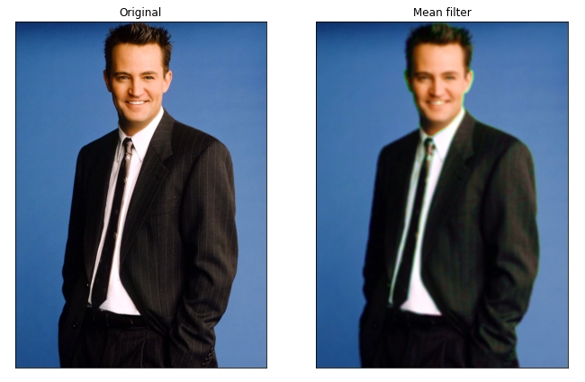
There are various techniques to remove noise from the image, technique depends on the type of noise present in the image. For salt and pepper noise, we use median filters, and for gaussian noise, we use mean filter (it smoothens the image).

We will talk about these techniques in the later part of the blog.

Applying Filter on an Image

Unfortunately, filters are a huge topic in image processing and it won't be possible to explain in this blog, But, if you want me to make a blog about Filters in Image Processing, Comment on this blog!!!

Here are some resources :

See video :

Filters on the image are applied using the convolution technique.

There are many types of filters used to sharpen or smoothen the image, edge detection, line detection, etc. (You can study these in Image Segmentation and in the later part of the chapter Intensity Transformations and Spatial Filtering).

Image Restoration

In Image Restoration, we talk about techniques used to remove/reduce noise from the input image (restoration of images).

Here, we will briefly talk about Mean Filter and Adaptive Median Filter.

• Mean Filter

There are various types of mean filters like arithmetic mean filter, geometric mean filter, harmonic filter, contraharmonic, and so on. The mean filter usually smoothens the image and is used to reduce gaussian noise in the image.

Arithmetic Mean Filter :

Here, g(x,y) is the image (which is degraded) and f(x,y) is the output image (which is not fully restored).

• Adaptive Median Filter

Adaptive Median Filter is used to remove salt and pepper noise from our input image. It works on the concept of median value in the kernel/window, here will do convolution on the input image, and for every (x,y) position we will replace the input value with the median value of the kernel/window. But, if we are not getting a good median value we increase the Kernel/Window Size for that (x,y) position, to get a better median value.

Code :

def fill_window(gray,x,y,windowSize):

    (rows,cols) = gray.shape
    window = np.zeros(windowSize*windowSize,dtype='uint8')
    halfSize = windowSize//2
    curr = 0

    # Uses Zero Padding
    for i in range(x-halfSize,x+halfSize+1):
        for j in range(y-halfSize,y+halfSize+1):
            if i<0 or i>=rows or j<0 or j>=cols:
                window[curr] = 0        # Zero Padding
            else:
                window[curr] = gray[i,j]
            curr += 1

    return window

# Apply this adaptive medain filter to reduce salt and pepper noise
def adaptive_median_filter(gray):

    def adaptive_median_filter_pixel(gray,x,y,windowSize):

        S_max = 21      # Maximum possible window size

        window = fill_window(gray,x,y,windowSize)

        z_min = int(np.min(window))
        z_max = int(np.max(window))
        z_median = int(np.median(window))
        z_xy = int(gray[x,y])

        # Level A
        a1 = z_median - z_min
        a2 = z_median - z_max

        if a1 > 0 and a2 < 0:
            # Level B
            b1 = z_xy - z_min
            b2 = z_xy - z_max

            if b1 > 0 and b2 < 0:
                res = z_xy
            else:
                res = z_median
        else:
            # Not getting a good value (window is small to analize)
            # Increasing Window Size
            windowSize += 2
            if windowSize > S_max:
                res = z_xy
            else:
                res = adaptive_median_filter_pixel(gray,x,y,windowSize)

        del window

        return res

    (rows,cols) = gray.shape

    # We will return this new image as output on this function
    filtered_img = np.zeros((rows,cols),dtype='uint8')

    # applying the adaptive median filter on each pixel
    for i in range(rows):
        for j in range(cols):
            filtered_img[i,j] = adaptive_median_filter_pixel(gray,i,j,3)        # initial window size in convolution as 3

    return filtered_img

Source

In this code, we have adaptive_median_filter_pixel function for applying this technique to get a new value at (x,y) position as output and adaptive_median_filter function will do convolution on the whole image and return the resulting image as output.

Color Images

There are mainly three types of Color Images type :

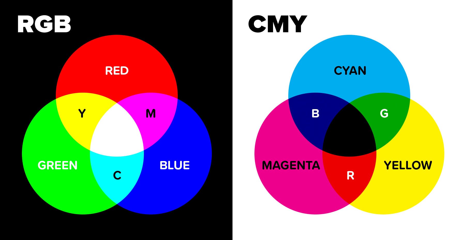
• RGB/BGR (Red, Green, Blue)

It is used for displaying images on a computer monitor or display, we can represent all colours using 3 values tuple (red, green, blue). Combining all red, green and blue we get white colour and pixel can easily show black colour by not lighting it up, it represents the black colour.

• CMY (Cyan, Magenta, Yellow)

It is used for printing, the reason for this is combining cyan, magenta and yellow we get black colour and as we know we give the white paper to the printer to print on it.

To convert RGB to CMY :

• HSI (Hue, Saturation, Intensity)

It is used for the manipulation of images, we will convert RGB to HSI then perform manipulations, and again convert to RGB for output.

Some code examples for you to study :

1. MATLAB Code Folder (Google Drive Link)

2. OpenCV Code Folder (Google Drive Link)

Interesting Facts :

• Lena Images

If we ever study or test your algorithms with the optimal results, you will surely see the example of the Lena image.

The "Lena" image is a well-known test image in image processing. Originally from Playboy magazine. Prized for its detail and range of tones, it's been used for decades to assess image processing algorithms. However, due to its source and ethical concerns, its use is becoming less common.

• Optical Illusions

I took this figure from the book mentioned in the introduction. This shows how our mind/brain perceives things, in the first and second images we see a square and a circle popping out of the image but it is just an illusion, similarly, the third image shows lines are of the same length but our brain perceives it differently because of arrows and the fourth image also shows parallel lines but we think they are not because of those strips on the line.

Conclusion

Now it's time to end this blog, hope you learned something from this blog.

It is a very basic blog on digital image processing and I have not covered many topics like image segmentation, morphological analysis, thresholding (dividing the image into foreground and background), etc. To study them you can read the book. Also, there are many free courses on YouTube and online provided by top universities. You can study this topic in those courses. It is a very interesting subject and the advanced level of this covers machine learning topics for image classification. The depth of this topic is endless and you can get a high-paying job in this subject.

If you want to study practice implementation, you can go through my code files mentioned above and read OpenCV documentation and MATLAB codes available on the internet.

Thank you for reading to the end! 🙌. You can contact me on Twitter(𝕏).